Sales Forecasting Project
This project focuses on forecasting weekly retail sales using the Walmart Store Sales dataset. The main objective is to predict future sales from historical store and department level data, with an emphasis on improving WMAE performance while keeping experiments reproducible and easy to compare through MLflow-tracked models, convergence plots, and feature engineering iterations. The Walmart forecasting task is a well-known Kaggle competition, and it’s useful as a realistic benchmark because it includes seasonality, promotions, holidays, and store-level heterogeneity. Sales behave very differently across departments and across stores (location, size, local demand), and the same calendar week can have completely different patterns depending on whether it contains a major holiday or a promotional period. That combination forces the model to learn both broad trends like global seasonality and highly local effects from stores, which is exactly what makes real retail forecasting challenging.
01 - Exploratory Data Analysis
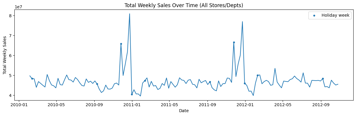
We start by joining the main training table (train.csv) with store metadata (stores.csv) and additional features (features.csv). The target is Weekly_Sales at the Store × Department × Week level, and the dataset includes a holiday flag (IsHoliday) and store attributes such as Type (A/B/C) and Size. To understand the global behavior, we aggregate Weekly_Sales across all stores and departments by week. Sales are fairly stable week-to-week, but there are sharp spikes at specific dates. Those spikes align with holiday weeks, confirming that holidays create large non-linear jumps in demand and justify using a holiday-weighted metric (WMAE) later. Next, we can look at average sales by week-of-year to see recurring patterns.
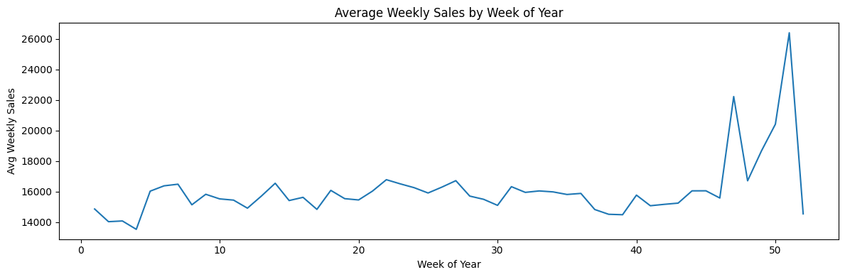
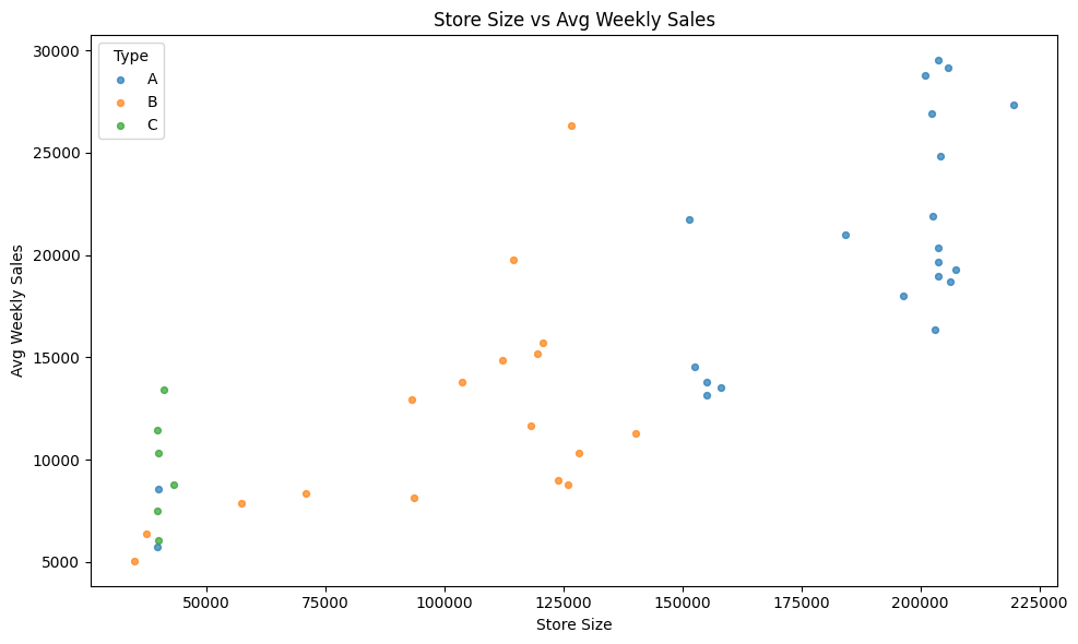
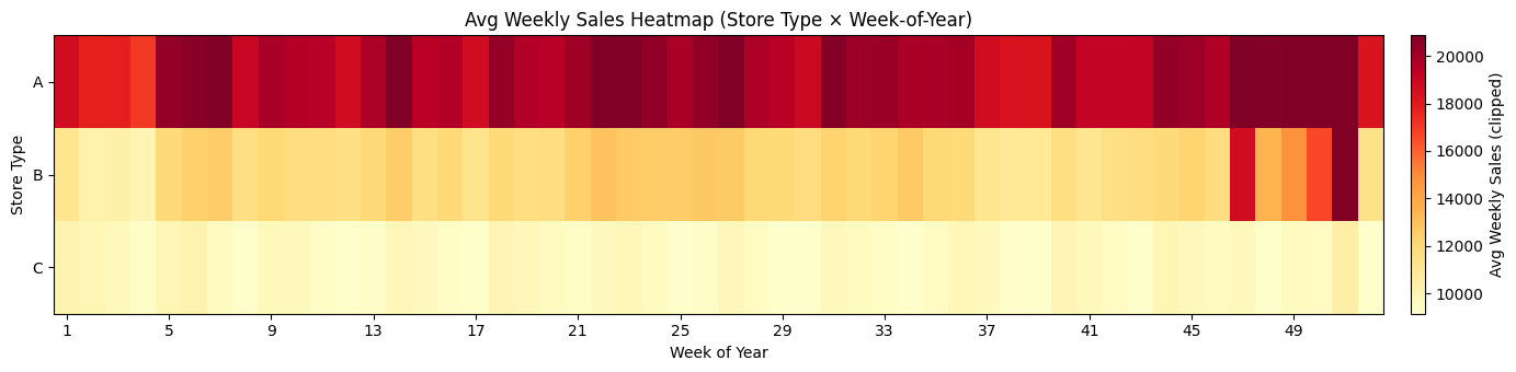
There is a clear seasonal structure throughout the year. The largest peaks occur in the final weeks (around weeks 47–52), consistent with major holiday shopping periods. This motivates feature engineering such as weekofyear, cyclical encodings (sin/cos), and lag/rolling history features which we can implement during training. Let us now examine hos store size relates to sales. Store Type A stores tend to be larger and achieve the highest average sales. Type B appears mid-sized with mid-range sales and type C clusters at smaller sizes and lower sales. This indicates store type and size are strong predictors and should be included directly in modeling. We can also compare seasonality patterns across store types using a heatmap of mean sales to confirm what we observed at the weekly level.
02 - Baseline Models
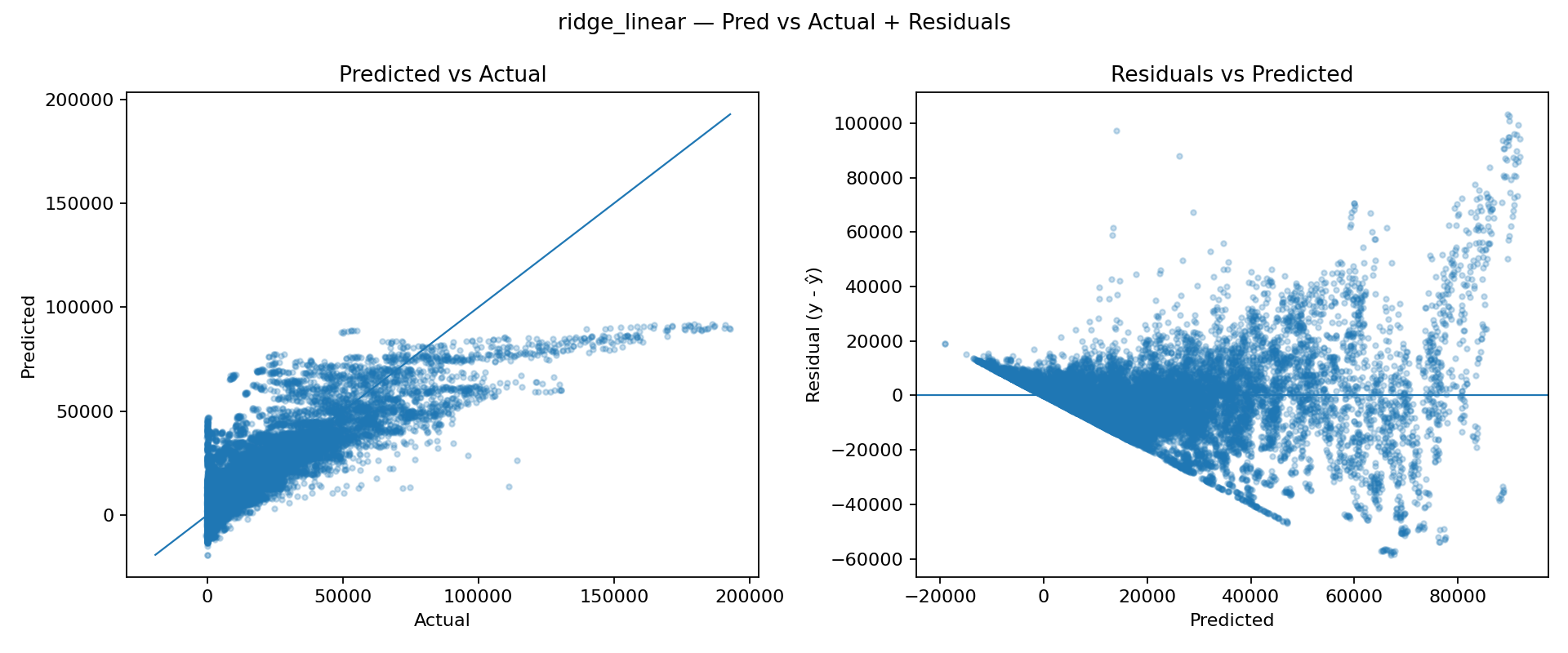
To establish a quick performance floor, we started with two simple baselines tracked in MLflow: a linear Ridge regression model and a Random Forest regressor. We first trained a Ridge model as a lightweight baseline. Since retail sales are driven by interactions (Store × Dept × seasonality × holidays), we expect the relationship to be strongly nonlinear, so Ridge is mainly useful as a sanity check. The Predicted vs Actual plot shows systematic underfitting (predictions compress into a narrow band). The residual plot reveals strong structure and heteroscedasticity (errors grow with the predicted value), indicating the model cannot represent the underlying patterns well.
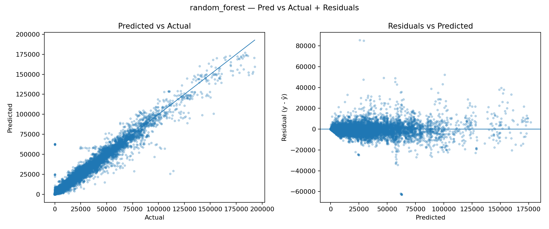
Next, we tested a Random Forest to introduce nonlinearity and feature interactions without heavy tuning. The Predicted vs Actual scatter aligns much more closely with the diagonal, showing a significantly better fit. Residuals are more centered around zero and less structured, suggesting the model is capturing nonlinear effects that Ridge cannot. These baselines confirm that the sales signal is highly nonlinear and benefits from models that can capture interactions and regime changes (e.g., store type, department, seasonality, and holiday behavior). While Random Forest is a strong sanity-check improvement, the next logical step is to move to gradient-boosted trees (XGBoost/LightGBM), which typically outperform bagging methods on tabular problems and offer better control over bias/variance trade-offs and training dynamics.
The results below compare the two baseline models across three evaluation metrics. Error-based metrics (WMAE and RMSE) should be minimized, whereas R² should be maximized. The Random Forest model provides the best overall performance on all three metrics. Next, we will train more promising models.
| Model | WMAE | RMSE | R² |
|---|---|---|---|
| ridge_linear | 7843.85 | 11896.36 | 0.7019 |
| random_forest | 1855.78 | 3795.73 | 0.9697 |
03 - More promising models
After validating that the problem is strongly nonlinear, we moved to gradient-boosted decision trees. This family of models is typically a strong fit for Walmart-style tabular data because it can represent complex interactions such as Store × Department effects, holiday behavior, and seasonal structure without requiring heavy feature scaling or strict parametric assumptions. Once the baseline solution with XGBoost was stable, the biggest jump in quality came from feature engineering designed to inject time-series memory into a tabular pipeline. The raw identifiers (Store, Dept, Type) are informative, but the sales process is also strongly driven by what happened recently in the same Store Dept pair. Adding lag features and rolling statistics (for example, last week's sales and short rolling means) is a fundamental step of modelling as it gives the model direct access to local dynamics that would otherwise require many trees to approximate indirectly.
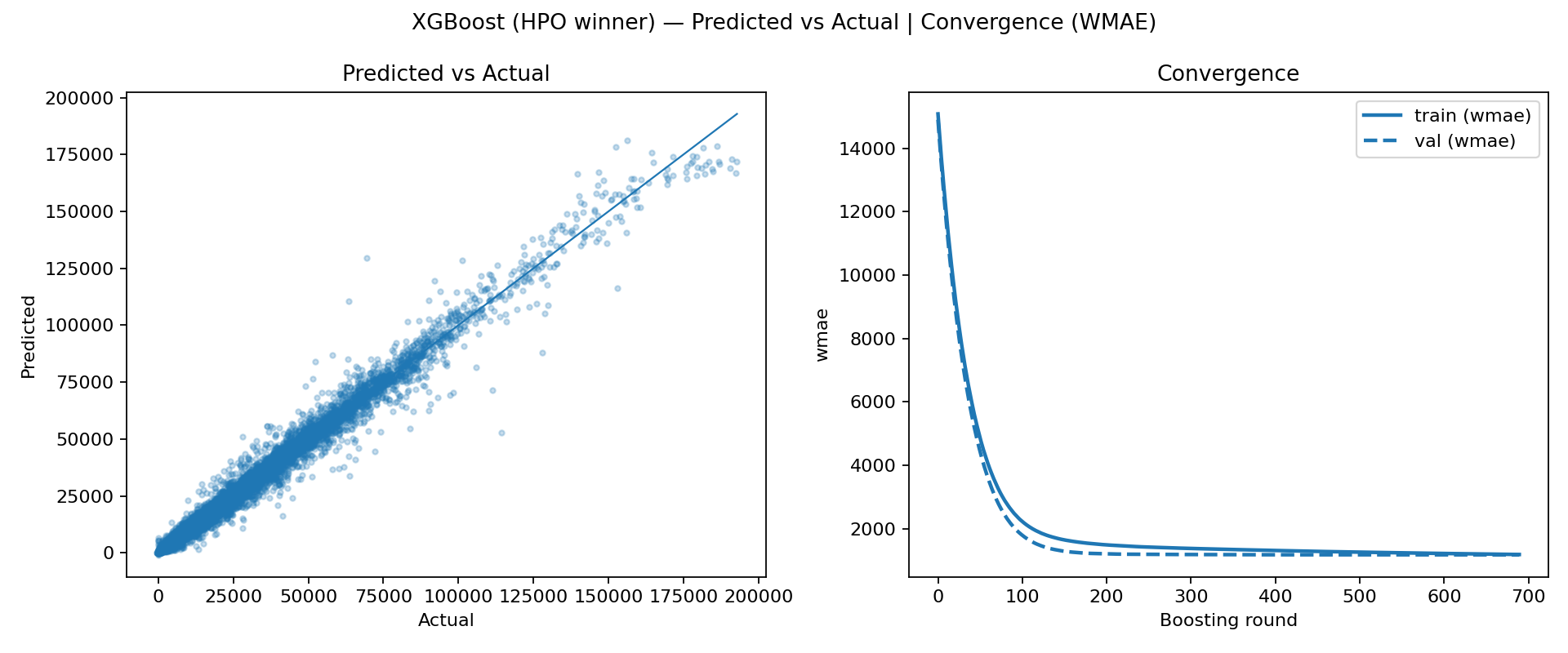
After adding these features, the model's behavior becomes more aligned with the underlying forecasting intuition: it can learn that the same department in the same store has a predictable baseline that changes smoothly over time, and it can adapt quickly when the recent history shifts. We then performed a quick hyperparameter optimization step to refine the learning rate, tree depth, and sampling/regularization settings. The resulting HPO winner convergence curve is especially informative: it drops very quickly and reaches a stable plateau within a smaller effective number of boosting rounds, which usually indicates a better bias variance trade-off and more efficient learning dynamics. In other words, the tuned configuration is not just fitting harder, it is fitting more cleanly, reaching a strong solution without needing thousands of marginally helpful trees.
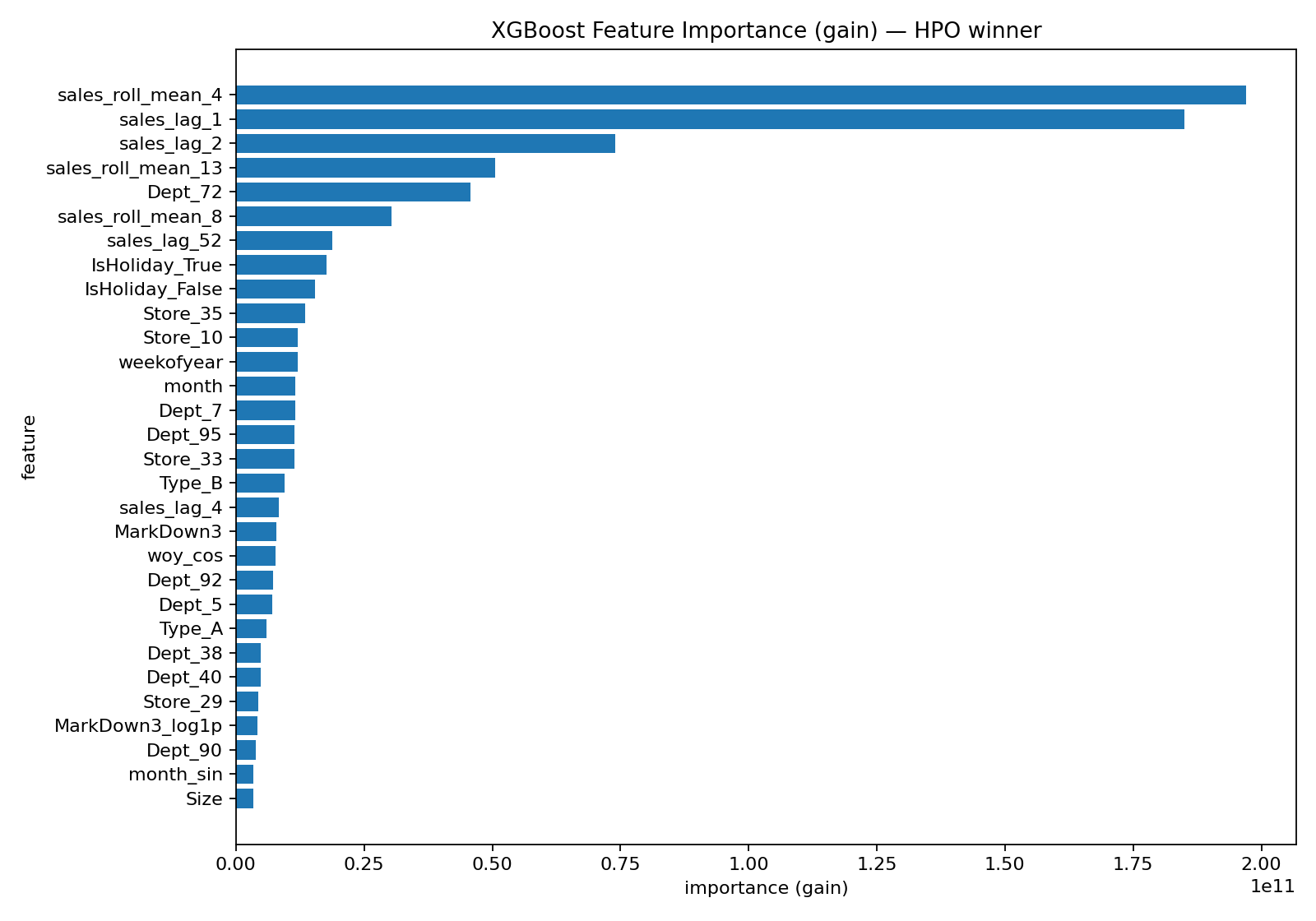
The feature-importance plot for the HPO winner helps confirm that the improvements came from the intended direction. Instead of the model relying primarily on static identifiers, the top-ranked features are dominated by lag and rolling history terms, meaning the model is using recent demand information as its primary signal. Holiday and calendar features still matter, as expected given the spikes seen in EDA, and store/dept indicators remain important as baseline anchors, but the key point is that the engineered temporal features now carry much of the predictive load.
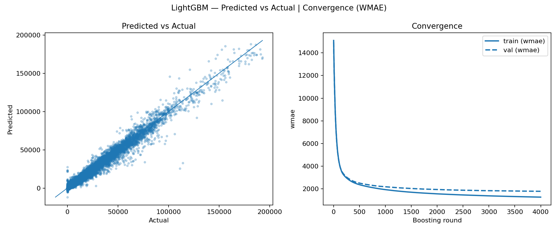
In parallel, we trained LightGBM using the same evaluation framework to compare performance and learning behavior. LightGBM also converges quickly, particularly on the training curve, which is consistent with its efficiency and strong default behavior on tabular datasets. However, in our runs it did not match XGBoost on validation performance, even though the model fit looked strong. Practically, this suggests that under the current preprocessing and feature set, XGBoost achieved a slightly better generalization trade-off, making it the more reliable choice as the leading model for the project. The table below summarizes the test-set performance of the main gradient-boosted models evaluated.
| model | WMAE | RMSE | R² |
|---|---|---|---|
| xgb_baseline | 1741.39 | 3095.29 | 0.9798 |
| xgb_hpo | 1232.70 | 2465.72 | 0.99 |
| lgbm_baseline | 1820.27 | 3264.60 | 0.9775 |
04 - State of the Art Models
After getting solid results with boosted trees, we wanted to see how far we could push things with modern time-series models. The big idea is that sales aren't just explained by store and department IDs plus calendar flags, they also have momentum, short-term memory, and recurring patterns that a sequence model might learn directly instead of us hand-feeding it lag features. We first tried an LSTM as a global model trained across many store/department series using a sliding window setup. It behaved the way you'd expect from a neural model on noisy retail data: it can definitely learn something meaningful, but training is more sensitive than XGBoost. The validation metric doesn’t improve in a clean, monotonic way, and it's easy to either underfit or start overfitting unless you're careful with scaling, window length, learning rate, and early stopping. It worked, and it was a useful checkpoint, but it didn’t beat the best boosted-tree runs in a consistent way.
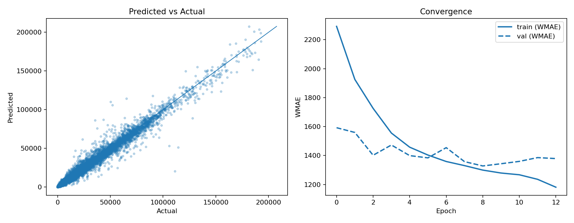
At that point we went looking for something more purpose-built for forecasting and ended up finding the N-BEATS paper. The architecture is nice because it's designed specifically around forecasting from history windows (backcast/forecast blocks), and it's widely used as a strong baseline in time-series work. We implemented a global N-BEATS model in PyTorch and trained it in the same global style across store/department series. We hit a couple practical issues along the way (the dataset has negative sales values due to returns, which breaks naive log transforms), so we used a signed log-style transform to keep training stable. After that, the model trained cleanly and we logged everything to MLflow with the same consistent artifacts: predicted vs actual, plus a validation WMAE curve per epoch.
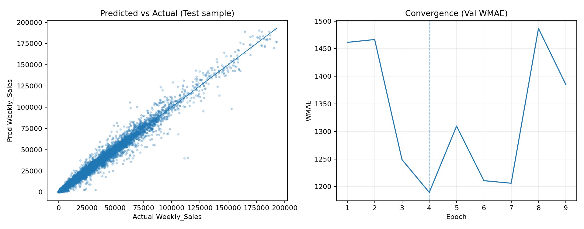
Surprisingly N-BEATS actually performed very well once the pipeline was fixed, albeit it doensn't converge quite the same way like other models. The scatter plot looked tight, and the final metrics were strong. The convergence curve looks different from XGBoost though, it's not the same kind of smooth, always-decreasing curve you get from boosting rounds, because neural nets train with mini-batch gradient descent and the validation metric can bounce around. That's normal, and it's why early stopping matters a lot more here. In the end, XGBoost with feature engineering and quick HPO still stayed the most dependable winner overall: stable training behavior, strong WMAE, and clear feature importance. But the LSTM and especially N-BEATS were great state-of-the-art experiments, and they show that with the right setup, a deep forecasting model can be competitive on this problem too.
| model | WMAE | RMSE | R² |
|---|---|---|---|
| lstm_baseline | 1517.39 | 3122.40 | 0.9803 |
| nbeats_global | 1211.81 | 2587.71 | 0.9850 |